Single Asset Risk: Standard Deviation and Coefficient of Variation
The return of any investment has an average, which is also the expected return, but most returns will differ from the average: some will be more, others, less. The more individual returns deviate from the expected return, the greater the risk and the greater the potential reward. The degree to which all returns for a particular investment or asset deviate from the expected return of the investment measures its risk.
Standard Deviation: Measure of Absolute Risk
If you recorded the returns of a sample population of investors who invested in 5-year Treasury notes (T-notes), you would note that everyone received a constant rate of return that didn't deviate, since, once bought, T-notes pay a constant rate of interest with no credit risk. On the other hand, if you had recorded the returns of a sample of investors who had invested in small stocks at the same time, you would see a much wider variation in their returns — some would have done much better than the T-note investors, while others would have done worse, and each of their returns would vary over time. This variability can be measured with statistical methods, because investment returns generally follow a normal distribution, which shows the probability of each deviation from the mean, which is the average return, or the expected return, for a particular asset.
The sum of the deviations, both positive and negative, forms a normal distribution about the mean. The normal distribution describes the variation of many natural quantities, such as height and weight. It also describes the distribution of investment returns. The normal distribution has the property that small deviations from the mean are more probable than larger deviations. When graphed, it forms a bell-shaped curve.
The mean is subtracted from each deviation, then squared to ensure that all deviations are positive numbers, then divided by the number of returns minus 1, which is the degrees of freedom for a small sample. This is called the variance. The square root of the variance is the standard deviation, which is simply the average deviation from the expected return. Standard deviations can measure the probability that a value will fall within a certain range. For normal distributions, 68% of all values will fall within 1 standard deviation of the mean, 95% of all values will fall within 2 standard deviations, and 99.7% of all values will fall within 3 standard deviations.
A normal distribution can be completely described by its mean and standard deviation. The extent of the deviation of investment returns is the volatility, measured by the standard deviation of the investment returns for a particular asset. Volatility differs according to the type of asset, such as stocks and bonds. Individual assets also differ in volatility, such as the stocks of different companies and bonds by different issuers. Volatility is commensurate with the investment's risk, and this risk can be quantified by calculating the standard deviation for particular investments, which is done by measuring the historical variation in the investment returns of particular assets or classes of assets. The greater the standard deviation, the greater the volatility, and, therefore, the greater the risk. More volatile assets have a wider bell-shaped curve, reflecting a greater dispersion in their returns. Likewise, 1 standard deviation will cover a wider dispersion of investment returns for a volatile asset than for a nonvolatile asset. Hence, more volatile assets are more likely to outperform or underperform less volatile assets.
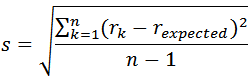 |
| s = Standard Deviation rk = Specific Return rexpected = Expected Return n = Number of Returns (sample size). |
Coefficient of Variation: Measure of Relative Risk
The greater the standard deviation, the greater the risk of an investment. However, the standard deviation cannot be used to compare investments unless they have the same expected return. For instance, consider the following table.
| Sample 1 | Sample 2 | |
|---|---|---|
| Return 11 | 6 | 9 |
| Return 2 | 4 | 11 |
| Return 3 | 6 | 9 |
| Return 4 | 4 | 11 |
| Expected Return | 5 | 10 |
| Standard Deviation | 1.154700538 | 1.154700538 |
| Coefficient of Variation | 0.230940108 | 0.115470054 |
On the left hand side, you have an investment with an expected return of $5 where each specific return deviates by $1 from the expected return. On the right hand side, the specific returns also deviate by $1, but the expected return is $10. Because the difference between the expected returns and the specific returns for each sample is 1, the standard deviation is the same, but, nonetheless, the risk is not the same, because $1 is only 10% of $10, but 20% of $5.
The coefficient of variation is a better measure of risk, quantifying the dispersion of an asset's returns in relation to the expected return, and, thus, the relative risk of the investment. Hence, the coefficient of variation allows the comparison of different investments.
Coefficient of Variation = Standard Deviation / Average Return
In the above case, both samples have the same standard deviation, but have a significant difference in the coefficient of variation. It is obvious that the investment with the smaller return has the greater risk in this case.
So while the standard deviation measures the dispersion of returns, the coefficient of variation measures their relative dispersion.
Example: Calculating the Standard Deviation and Coefficient of Variation
Using the data from Sample 1 in the above table, where the average or expected return = 5, and the formulas for the standard deviation and coefficient of variation and remembering that x1/2 = √x, we find that:
| Standard Deviation Using Microsoft Excel Coefficient of Variation | = ((6 - 5)2 + (4 - 5)2 + (6 - 5)2 + (4 - 5)2 / 4 - 1)1/2 = (4/3)1/2 = 1.154700538 = STDEV(6,4,6,4) = 1.154700538 = 1.154700538 / 5 = 0.230940108 |
Microsoft Excel also has a function to calculate the standard deviation, STDEV, using the format STDEV(number 1, number 2, ...), an example calculation is also shown in the above table for Sample 1. You can also select the numbers in the table as the input to the STDEV function. There is no Excel function for the coefficient of variation, but it is simple enough to calculate, knowing the standard deviation.