Modern Portfolio Theory: Efficient and Optimal Portfolios
A portfolio consists of different securities or other assets selected for investment gains. However, a portfolio also has investment risks. The primary objective of portfolio theory or management is to maximize gains while reducing diversifiable risk. Diversifiable risk is so named because the risk can be reduced by diversifying assets. Systemic risk, on the other hand, cannot be reduced through diversification since it is a risk that affects the entire economy and most investments. So even the most optimized portfolio will still be subject to systemic risk.
Traditional portfolio management is a nonquantitative approach to balancing a portfolio with different assets, such as stocks and bonds, from different companies and different sectors to reduce overall risk of the portfolio. The main objective is to select assets with little or negative correlation with each other, so that the overall diversifiable risk is reduced.
Modern portfolio theory (MPT) reduces portfolio risk by selecting and balancing assets based on statistical techniques that quantify the amount of diversification by calculating expected returns, standard deviations of individual securities to assess their risk, and by calculating the actual coefficients of correlation between assets, or by using a good proxy, such as the single-index model, allowing a better choice of assets with negative or no correlation with other assets in the portfolio. Modern portfolio management differs from the traditional approach by using quantitative methods to reduce risk. The main objective of modern portfolio theory is to have an efficient portfolio, which is a portfolio that yields the highest return for a specific risk, or, stated in another way, the lowest risk for a given return. Profits can be maximized by selecting an efficient portfolio that is also an optimal portfolio, which provides the most satisfaction — the greatest return — for an investor based on his tolerance for risk.
Efficient Frontier
Because portfolios can consist of any number of assets with differing proportions of each asset, risk-return ratios vary widely. If the universe of these risk-return possibilities — the investment opportunity set — were plotted as an area of a graph with the expected portfolio return on the vertical axis and portfolio risk on the horizontal axis, the entire area would consist of all feasible portfolios — those that are actually attainable. In this set of attainable portfolios, there would be some which have the greatest return for each risk level, or, for each risk level, there would be portfolios with the greatest return. The efficient frontier is the set of all efficient portfolios yielding the highest return for each level of risk. The efficient frontier can be combined with an investor's utility function to find the investor's optimal portfolio, the portfolio with the greatest return for the risk that the investor is willing to accept.

On the efficient frontier, there is a portfolio with the minimum risk, as measured by the variance of its returns — hence, it is called the minimum variance portfolio — that also has a minimum return, and a maximum return portfolio with a concomitant maximum risk. Portfolios below the efficient frontier offer lower returns for the same risk, so a wise investor would not choose such portfolios.
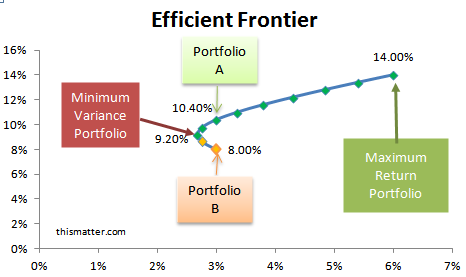
Below is a diagram constructed by combining 2 assets into various portfolios by changing the weighting for each asset in each portfolio. :
Asset A
- expected return = 14%
- standard deviation = 6%
Asset B
- expected return = 8%
- standard deviation = 3%
All the portfolios consisting of these 2 assets lie on the graph below, which is the investment opportunity set. The efficient frontier extends from the minimum variance portfolio to the maximum return portfolio. Two portfolios lie below the efficient frontier. These 2 portfolios will yield a smaller return for the same risk as those on the efficient frontier. For instance, if an investor did not want to assume any greater risk than that offered by Portfolio A and Portfolio B, then the investor would choose Portfolio A over B, because both have the same risk, but Portfolio A returns 10.4% while Portfolio B returns only 8%. Portfolio B consists only of Asset B; the maximum return portfolio consists only of Asset A. Note that the minimum variance portfolio not only has a greater expected return, but also a lower risk than a portfolio consisting only of Asset B.
Utility Values and Risk Aversion
Most investors will assume a greater risk for a greater return. However, investors differ in the amount of risk they are willing to take for a given return. Investors who are risk averse require a greater return for a given amount of risk than a risk lover. A risk-neutral investor is only concerned with the magnitude of the return. However, most investors are risk averse to varying degrees.
Though investors differ in their risk tolerance, they should be consistent in their selection of any portfolio in terms of the risk-return trade-off. Because risk can be quantified as the sum of the variance of the returns over time, it is possible to assign a utility score (aka utility value, utility function) to any portfolio by subtracting its variance from its expected return to yield a number that would be commensurate with an investor's tolerance for risk, or a measure of their satisfaction with the investment. Because risk aversion is not an objectively measurably quantity, no unique equation would yield such a quantity, but an equation can be selected, not for its absolute measure, but for its comparative measure of risk tolerance. One such equation is the utility formula:
Utility Score = Expected Return − 0.005σ2 × Risk Aversion Coefficient
The risk aversion coefficient is a number proportionate to the amount of risk aversion of the investor and is usually set to integer values less than 6, and 0.005 is a normalizing factor to reduce the size of the variance, σ2, which is the square of the standard deviation (σ), a measure of the volatility of the investment and therefore its risk. This equation is normalized so that the result is a yield percentage that can be compared to investment returns, which allows the utility score to be directly compared to other investment returns, such as the return of risk-free T-bills. Example: if a risk-free T-bill pays 4%, and JXYZ stock returns 12% with a standard deviation of 25%, then the utility score of JXYZ stock is calculated thus:
Utility Score = 12 − 0.005 × 252 × 2
- = 12 − 6.25 = 5.75%
In the above example, we let the risk aversion coefficient be equal to 2. If someone were more risk averse, we might use 3 instead of 2 to indicate the investor's greater aversion to risk. In this case, the above equation yields:
Utility Score = 12 − 0.005 × 252 × 3
- = 12 − 9.375 = 2.625%
Since 2.625% is less than the 4% yield of risk-free T-bills, this risk-averse investor will reject JXYZ stock for T-bills while the other investor will invest in JXYZ stock since he assigns a utility score of 5.75% to the investment, which exceeds the T-bill yield.
Another way to measure the risk averseness of an investor is by comparing the desirability of a risky investment to a risk-free investment. The certainty equivalent rate is the rate of return of a risk-free investment that would be equally attractive as a risky investment. Since the utility score of a risk-free investment is simply its rate of return (in other words, the variance of a risk-free investment is considered zero, hence the 2nd term of the utility score formula is zero), the certainty equivalent rate would equal the utility score of the risky investment. So for the 1st investor above, a risk-free yield of 5.75% would be equally attractive as JXYZ stock yielding a risky 12%, while the 2nd investor would only consider JXYZ stock if the risk-free rate were only 2.625%. In other words, each investor would be indifferent to either investment if the risk-free rate were equal to their certainty equivalent rate.
The set of all portfolios with the same utility score plots as a risk-indifference curve. An investor will accept any portfolio with a utility score on her risk-indifference curve as being equally acceptable.

However, many possible portfolios on many risk-indifference curves do not yield the highest return for a given risk. All of these portfolios lie below the efficient frontier. The optimal portfolio is a portfolio on the efficient frontier yielding the best combination of return and risk for a given investor, giving that investor the most satisfaction.

In the graph below, risk-indifference curves are plotted along with the investment opportunity set of attainable portfolios. Data points outside of the investment opportunity set designate portfolios that are not attainable, while those portfolios that lie along the northwest boundary of the investment opportunity set is the efficient frontier. All portfolios that lie below the efficient frontier have a risk-return trade-off that is inferior to those that lie on the efficient frontier. If a utility curve intersects the efficient frontier at 2 points, portfolios on the same curve that lie below the efficient frontier are not optimal. Remember that all points on a risk-indifference curve are equally attractive to the investor; therefore, if any points on the indifference curve lie below the efficient frontier, then no point on that curve can be an optimum portfolio for the investor. A utility curve that lies wholly above the efficient frontier has no attainable portfolio.
However, a utility curve intersects the efficient frontier at a single point — this is the optimum portfolio. The only attainable portfolio is on the efficient frontier, and thus, provides the greatest satisfaction to the investor. The optimum portfolio will yield the highest return for the amount of risk that the investor is willing to take.

Portfolio Betas: A Measure of the Systemic Risk of Portfolios
By selecting the right assets in the right proportions, it may be possible to reduce diversifiable risk to near zero, but the portfolio would still have systemic risk, which also affects the general market. Portfolios, like stocks, have betas which measure the systemic risk of the portfolio compared to that of the market. The portfolio beta = the sum of the beta of the weighted average of each security's value over the portfolio value.
| Portfolio Beta | = | n ∑ k=1 | Dollar Amount of Asset k Dollar Amount of Portfolio | × | Beta for Asset k |
Example: Calculating the Portfolio Beta
You can find the beta of most stocks at websites providing stock quotes. What is the beta of this portfolio consisting of 100 shares of each stock?
- Stock 1
- Share Price: $20.88
- Beta: 0.99
- Stock 2
- Share Price: $331.22
- Beta: 1.55
- Total Portfolio Value
- = $20.88 × 100 + $331.22 × 100
- = $2,088 + $33,122
- = $35,210
Portfolio Beta
- = $2,088/$35,210 × 0.99 + $33,122/$35,210 × 1.55
- = 0.06 + 1.46 = 1.52
Hence, this portfolio would be 1.5 times as volatile as the S&P 500 index, which is considered to have a beta of 1. When the S&P rises by 1%, this portfolio tends to increase by 1.5%; when the S&P is down 1%, this portfolio will likely be down 1.5%. Remember that since the beta is a statistical value, actual ratios will deviate frequently from these values.
The portfolio beta is interpreted like it is for stocks. A portfolio with a beta of 1 has the volatility of the stock market — the value of the portfolio moves 1%, up or down, for each 1% move in the stock market; a portfolio beta value of 0.5 would have half the volatility of the market and a beta of 2 would have twice the volatility.
Hence, the portfolio beta allows an investor to choose securities or other assets that would limit the investor's exposure to systemic risk to her risk tolerance.
Utility Theory is Based on Rationality
Utility theory, and indeed, most of economics is based on the rational economic man, where individuals always act rationally and would choose the best outcomes. However, people often make irrational decisions. While utility theory provided excellent insights into how an investor would choose rationally, irrationality is harder to study, but becomes more important amid uncertainty. New developments in economics, especially behavioral economics, is tackling these obstacles to gain a more complete picture of how people actually act and choose.